Introduction
Often, a longer document contains many themes, and each theme is located in a particular segment of the document. For example, each paragraph in a political essay may present a different argument in support of the thesis. Some arguments may be sociological, some economic, some historical, and so on. Thus, themes vary across the document, but remain constant within each segment. We will call such segments "coherent".
This post describes a simple principle to split documents into coherent segments, using word embeddings. Then we present two implementations of it. Firstly, we describe a greedy algorithm, which has linear complexity and runtime in the order of typical preprocessing steps (like sentence splitting, count vectorising). Secondly, we present an algorithm that computes the optimal solution to the objective given by the principle, but is of quadratic complexity in the document lengths. However, this optimal algorithm can be restricted in generality, such that processing time becomes linear.
The approach presented here is quite similar to the one developed by Alemi and Ginsparg in Segmentation based on Semantic Word Embeddings.
The implementation is available as a module on GitHub.
Preliminaries
In the discussion below, a document means a sequence of words, and the goal is to break documents into coherent segments. Our words are represented by word vectors. We regard segments themselves as sequences of words, and the vectorisation of a segment is formed by composing the vectorisations of the words. The techniques we describe are agnostic to the choice of composition, but we use summation here both for simplicity, and because it gives good results. Our techniques are also agnostic as to the choice of the units constituting a document -- they do not need to be words as described here. Given a sentence splitter, one could also consider a sentence as a unit.
Motivation
Imagine your document as a random walk in the space of word embeddings. Each step in the walk represents the transition from one word to the next, and is modelled by the difference in the corresponding word embeddings. In a coherent chunk of text, the potential step directions are not equally likely, because word embeddings capture semantics, and the chunk covers only a small number of topics. Since only some step directions are likely, the length of the accumulated step vector grows more quickly than for a uniformly random walking direction.
Remark: Word embeddings usually have a certain preferred direction. One survey about this and a recipe to investigate your word embeddings can be found here.
Formalisation
Suppose $V$ is a segment given by the word sequence $(W_1, ... W_n)$ and let $w_i$ be the word vector of $W_i$ and $v := \sum_i w_i$ the segment vector of $V$.
The remarks in the previous section suggest that the segment vector length $\|v\|$ corresponds to the amount of information in segment $V$. We can interpret $\|v\|$ as a weighted sum of cosine similarities:
\[\|v\| = \left\langle v, \frac{v}{\|v\|} \right\rangle = \sum_i\left\langle w_i, \frac{v}{\|v\|}\right\rangle = \sum_i \|w_i\|\left\langle \frac{w_i}{\|w_i\|}, \frac{v}{\|v\|}\right\rangle.\]
As we usually compare word embeddings with cosine similarity, the last scalar product $\left\langle \frac{w_i}{\|w_i\|}, \frac{v}{\|v\|}\right\rangle$ is just the similarity of a word $w_i$ to the segment vector $v.$ The weighting coefficients $\| w_i \|$ suppress frequent noise words, which are typically of smaller norm. So $\|v\|$ can be described as accumulated weighted cosine similarity of the word vectors of a segment to the segment vector. In other words: the more similar the word vectors are to the segment vector, the more coherent the segment is.
How can we use the above notion of coherence to break a document of length $L$ into coherent segments, say with word boundaries given by the segmentation:
\[T := (t_0, ..., t_n) \quad \text{such that} \quad 0 = t_0 < t_i < ... < t_n = L\]
A natural first attempt is to ask for $T$ maximising the sum of segment vector lengths. That is, we ask for $T$ maximising:
\[ J(T) := \sum_{i=0}^{n-1}\left\| v_i \right\|, \quad \text{where} \; v_i := w_{t_i} + \ldots + w_{t_{i+1} - 1}.\]
However, without further constraints, the optimal solution to $J$ is the partition splitting the document completely, so that each segment is a single word. Indeed, by the triangle inequality, for any document $(W_0, ..., W_{L-1})$, we have:
\[ \left\| \sum_{i=0}^{L-1} w_i \right\| \le \sum_{i=0}^{L-1} \| w_i \|. \]
Therefore, we must impose some limit on the granularity of the segmentation to get useful results. To achieve this, we impose a penalty for every split made, by subtracting a fixed positive number $\pi$ for each segment. The error function is now:
\[ J(T) := \sum_{i=0}^{n-1} \left( \left\| v_i \right\| - \pi \right).\]
Algorithms
We developed two algorithms to tackle the problem. Both depend on a hyperparameter, $\pi$, that defines the granularity of the segmentation. The first one is greedy and therefore only a heuristic, intended to be quick. The second one finds an optimal segmentation for the objective $J$, given split penalty $\pi$.
Greedy
The greedy approach tries to maximise $J(T)$ by choosing split positions one at a time.
To define the algorithm, we first define the notions of the gain of a split, and the score of a segmentation. Given a segment $V = (W_b, \ldots, W_{e-1})$ of words and a split position $t$ with $b<t<e$, the gain of splitting $V$ at position $t$ into $(W_b, \ldots, W_{t-1})$ and $(W_t, \ldots, W_{e-1})$ is the sum of norms of segment vectors to the left and right of $c$, minus the norm of the segment vector $v$:
\[ {gain}_b^e(t) := \left\| \sum_{i=b}^{t-1} w_i \right\| +\left\| \sum_{i=t}^{e-1} w_i \right\| -\left\| \sum_{i=b}^{e-1} w_i \right\|\]
The score of a segmentation is the sum of the gains of its split positions.
\[ {score}(T) := \sum_{i=1}^{n-1} {gain}_{t_{i-1}}^{t_{i+1}}(t_i)\]
The greedy algorithm works as follows: Split the text iteratively at the position where the score of the resulting segmentation is highest until the gain of the latest split drops below the given penalty threshold.
Note that the splits resulting from this greedy approach may be less than the penalty $\pi$, implying the segmentation is sub-optimal. Nonetheless, our empirical results are remarkably close to the global maximum of $J$ that is guaranteed to be achieved by the dynamic programming approach discussed below.
Dynamic Programming
This approach exploits the fact that the optimal segmentations of all prefixes of a document up to a certain length can be extended to an optimal segmentation of the whole. The idea of dynamic programming is that one uses intermediate results to complete a partial solution. Let's have a look at our case:
Let $T := (t_0, t_1, ..., t_n)$ be the optimal segmentation of the whole document. We claim that $T' := (t_0, t_1, ..., t_k)$ is optimal for the document prefix up to word $W_k.$ If this were not so, then the optimal segmentation for the document prefix $(t_0, t_1, t_2, ..., t_k)$ would extend to a segmentation $T''$ for the whole document, using $t_{k+1}, ..., t_n$, with $J(T'') < J(T)$, contradicting optimality of $T$. This gives us a constructive induction: Given optimal segmentations
\[\{T^i \;|\; 0 < i < k, \;T^i \;\text{optimal for first} \;i\; \text{words}\},\]
we can construct the optimal segmentation $T^k$ up to word $k$, by trying to extend any of the segmentations $T^i, \;0 < i < k$ by the segment $(W_i, \ldots W_k)$, then choosing $i$ to maximise the objective. The reason it is possible to divide the maximisation task into parts is the additive composition of the objective and the fact that the norm obeys the triangle inequality.
The runtime of this approach is quadratic in the input length $L$, which is a problem if you have long texts. However, by introducing a constant that specifies the maximal segment length, we can reduce the complexity to merely linear.
Hyperparameter Choice
Both algorithms depend on the penalty hyperparameter $\pi$, which controls segmentation granularity: The smaller it is, the more segments are created.
A simple way of finding an appropriate penalty is as follows. Choose a desired average segment length $m$. Given a sample of documents, record the lowest gains returned when splitting each document iteratively into as many segments as expected on average due to $m$, according to the greedy method. Take the mean of these records as $\pi$.
Our implementation of the greedy algorithm can be used to require a specific number of splits and retrieve the gains. The repository comes with a get_penalty function that implements the procedure as described.
Experiments
As word embeddings we used word2vec cbow hierarchical softmax models of dimension 400 and sample parameter 0.00001 trained on our preprocessed English Wikipedia articles.
$P_k$ Metric
Following the paper Segmentation based on Semantic Word Embeddings, we evaluate the two approaches outlined above on documents composed of randomly concatenated document chunks, to see if the synthetic borders are detected. To measure the accuracy of a segmentation algorithm, we use the $P_k$ metric as follows.
Given any positive integer $k$, define $p_k$ to be the probability that a text slice $S$ of length $k$, chosen uniformly at random from the test document, occurs both in the $i^{{th}}$ segment of the reference segmentation and in the $i^{{th}}$ segment the segmentation created by the algorithm, for some $i$, and set
\[P_k := 1 - p_k.\]
For a successful segmentation algorithm, the randomly chosen slice $S$ will often occur in the same ordinal segment of the reference and computed segmentation. In this case, the value of $p_k$ will be high, hence the value of $P_k$ low. Thus, $P_k$ is an error metric. In our case, we choose $k$ to be one half the length of the reference segment. We refer to the paper for more details on the $P_k$ metric.
Test documents were composed of fixed length chunks of random Wikipedia articles that had between 500 and 2500 words. Chunks were taken from the beginning of articles with an offset of 10 words to avoid the influence of the title. We achieved $P_k$ values of about 0.05. We varied the length of the synthetic segments over values 50, 100 or 200 (the vertical axis in the displayed grid). We also varied the number of segments over values 3, 5 and 9 (the horizontal axis).
Our base word vectorisation model was of dimension 400. To study how the performance of our segmentation algorithm varied with shrinking dimension, we compressed this model, using the SVD, into 16, 32, 64 and 128-dimensional models, and computed the $P_k$ metrics for each. To do this, we used the python function:
<pre>
def reduce(vecs, n_comp):
u, s, v = np.linalg.svd(vecs, full_matrices=False)
return np.multiply(u[:, :n_comp], s[:n_comp])
</pre>
The graphic shows the $P_k$ metric (as mean) on the Y-axis. The penalty hyperparameter $\pi$ was chosen identically for both approaches and adjusted to approximately retrieve the actual number of segments.
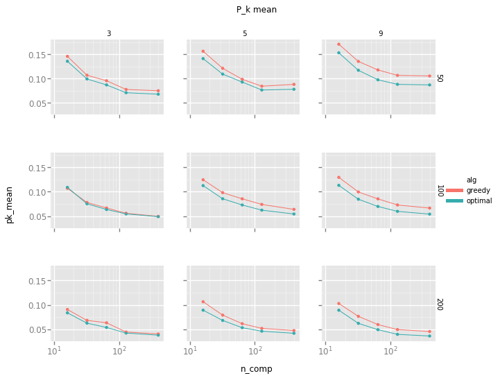
Observations:
- The dimension reduction is efficient, as runtime scales about linearly with dimension, but perfect accuracy is still not reached for 128 dimensions.
- The metric improves with the length of the segments. Perhaps this is because the signal to noise ratio improves similarly.
Since both our segmentation test corpus and word embedding training corpus are different from those of Alemi and Ginsprang, our $P_k$ values are not directly comparable. Nonetheless, we observe that our results roughly match theirs.
Runtime
Experiments were done on 2.4 GHz CPU. We see the runtime properties claimed above, as well as the negligible effect of the number of segments for fixed document length.
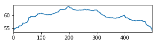
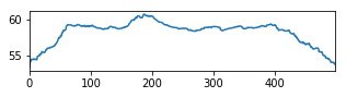
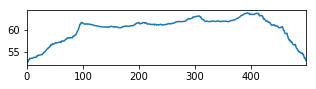
Greedy Objective
The graph shows the objective maximized in the first step of the greedy algorithm. Each graph is a synthetic document composed of 5 chunks of length 100 each. The peaks at multiples of 100 are easy to spot.
Application to Literature
In this section, we apply the above approach to two books. Since the experiment is available as jupyter-notebook, we omit the details here. The word vectors are trained on a cleaned sample of the english Wikipedia with 100 MB compressed size (see here).
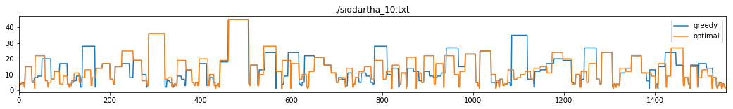
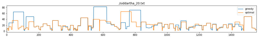
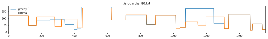
We run the two algorithms on the books Siddartha, by Hermann Hesse and A tale of two cities, by Charles Dickens. We use sentences in place of words and sentence vectors are formed as the sum of word vectors of the sentence. The penalty parameter for the optimal method was determined for an average segment length of 10, 20, 40 and 80 sentences through the get_penalty method. (Notice that this results not in these exact average segment lengths, as can be seen in the notebook outputs). The greedy method was parametrised to produce the same number of splits as the optimal one, for better comparison. The graphics show sentence index on the x-axis and segment length on the y-axis. The text files with sentence and segment markers are also available.
siddartha_10.txt siddartha_20.txt siddartha_40.txt siddartha_80.txt

tale2cities_10.txt tale2cities_20.txt tale2cities_40.txt tale2cities_80.txt
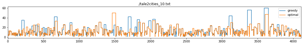
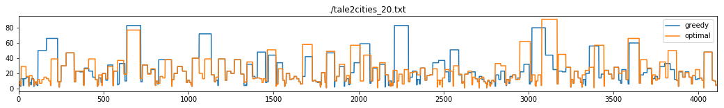
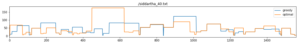
The segmentations derived by both methods are visibly similar, given the overlapping vertical lines. The values of the associated objective functions differ only by ~0.1 percent.
The segmentation did not separate chapters of the books reliably. Nevertheless, there is a correlation between chapter borders and split positions. Moreover, in the opinion of the author, neighbouring chapters in each of the above books often contain similar content.
We also did experiments with nonnegative word embeddings coming from a 25-dimensional NMF topic model, trained on TfIdf vectorisations of sentences from each text. Our results were of similar quality to those reported here. One advantage of this approach is that there are no out-of-vocabulary words, a particular problem in the case of specific character and place names.
Discussion
The two segmentation algorithms presented here -- each using precomputed word embeddings trained on the English Wikipedia corpus -- both performed very well with respect to the $P_k$ metric on our test corpus of synthetically assembled Wikipedia article chunks. Determining whether these algorithms perform well in more realistic scenarios in other knowledge domains would require annotated data.
For practical purposes, it might be disturbing that the variance in segment length is quite large. This can probably be tackled by smoothing the word vectors with a window over neighbouring words.